MRI Tissue Contrast
I have thought a lot about how an MRI scan with all its sequences could be distilled down to a short simple explanation to no avail. The questions radiology trainees ask themselves while reading these studies such as “Just what is T1 and T2?”, “Why does it seems so blurry compared to CT?”, “What causes this artifact?” (for a few examples) take a long time to answer if your starting point is: I know MRI has A) something to do with magnets and protons and B) the machine looks sort of like a CT scanner. There’s no shame in being at that level of knowledge (OK, maybe a little). MRI is an easy topic to keep putting off since understanding how it works isn’t required for interpreting most of the images.
This post is an attempt to answer the tissue contrast question (“What is T1 and T2?”). I think it will be the first of a series of posts explaining aspects of MRI. First, however, we need a high-level overview of the machine to frame the discussion. For the overview, I am leaving out many, many details to ensure the gist and relevant bits for a radiologist are not lost. Don’t send me hate mail please.
The big picture
The MRI scanner looks like a CT scanner but does not function at all like a CT scanner. That is, a CT scan internally is something like the C-arm x-ray machine in the IR suite, except spinning around really fast. The CT’s computer records the x-rays hitting the detector plate as a function of angle and time. This gives you a big dataset to which some algorithms are applied, generating our familiar axial, sagittal and coronal series. Fundamentally though, CT is x-ray technology and x-ray physics.
Even though the MRI is a cylinder that the patient goes into like a CT, there is no moving source beam of x-rays, protons, radio-waves, or of anything similar. There is no detector plate. The machine is physically a big ring of metal with some stationary wiring and cooling solution. The patient may wear a “coil”, which you should think of like a car radio or cellphone antenna, which records the signal. Alternatively, the receiver may be within the machine itself. Like your cellphone, the receiver is going to get better reception closer to the target organs. That’s why we have a knee coil, head coil, body coil, and so on.
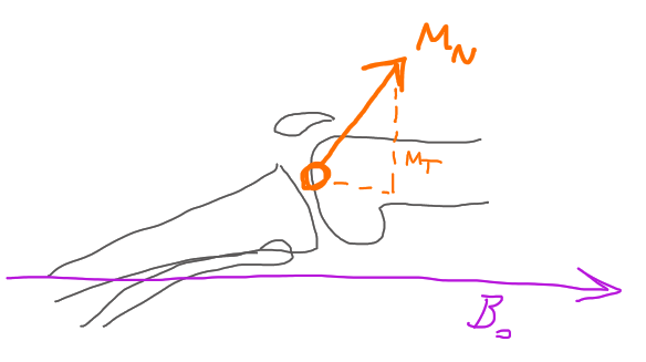
The main electromagnet is always on, generating a strong unchanging magnetic field (called B0). This field induces a much smaller magnetic field in the patient called net magnetization (MN) when the patient enters the bore. The machine then generates a brief resonant radiofrequency (RF) pulse. This reorients the patient’s body’s magnetic field (MN) such that it can be measured. Milliseconds after the pulse, the patient’s magnetic field strength is measured. The measured data itself is a short digital 2D signal vs time waveform. This process repeats many times—let’s say for the sake of this example–128 times to generate one image of one series.
At specific times before each measurement, small gradient magnetic fields are produced by the machine and are used to manipulate the patient’s body’s magnetic field a bit. This changes the signal that is measured, and these small adjustments are ultimately used by the computer to divide the signal up in 3D space (among other things). Without the gradients, we would just be measuring the same thing over and over. Once enough data is collected, algorithms are used to produce a picture. Altogether, this is a time consuming process, and now you can see why it takes 40 minutes to do an MRI scan.
The specific timed pattern we use (one or more pulses, turning gradients on and off, recording data, and repeating the process) defines what we call a “sequence”. Sequences names are familiar to you even if you don’t know what they mean yet. Example names are gradient recalled echo (GRE), fast-spin-echo (FSE), and short tau inversion recovery (STIR), which are defined by the sequence of events used to acquire the data for the picture.
Sequence types may be further subdivided by a “weighting”, called T1, T2, and proton density. As you know, this can dramatically change the appearance of the image–something dark on one series becomes bright on another. Practically, the difference between these three weightings is merely a matter of timing—when you measure the signal (called echo time [TE]) and when you repeat your sequence (repetition time [TR]). These times in milliseconds probably show up as a text overlay in one of the corners of the MRI image you are looking at.
Each of the last five paragraphs could easily be expanded into full lectures. How do we induce a magnetic field in some tissue? How do we manipulate that field? How do we measure it? How do we spatially subdivide the measured signal? How are the sequences different? What is T1 and T2 weighting? Answering that last question is the purpose of this post.
Magnetic properties of tissue
For example imagine or refer to a Knee MRI. The question we want to answer here is “Why is one pixel of joint fluid on the T1 image dark when roughly the same pixel location of joint fluid on the T2 image is bright?” At the same time, the bone marrow and subcutaneous fat are bright on both images. The air and periosteum are dark on both images.
At the time of measurement, the machine measures the vector component of net magnetization of the entire patient that is not in the same plane with the main magnetic field, called transverse magnetization (MT). Imagine that your measurement results in a single value. I am going to completely make this value up. We measured the patient and got 5 Amperes of induced current in our receiver coil. This measurement contains contributions from all the tissue at once. Mathematical wizardry will be used to divide up the signal spatially, but that is a big topic for another article. For our purposes today, imagine you are just putting a big slab of fat or a large flask of joint fluid in the machine and measuring it. The final pixel value brightness on the image corresponds to the amplitude of our MT measurement.

A slab of fat has various intrinsic properties which are based entirely on its composition and structure. It has a mass. It has a certain number of atoms. It has a volume. A few of these intrinsic properties were invented to describe how a particular object behaves in an MRI machine. First, every tissue has a proton density (PD), which represents the number of protons which are available to contribute to the signal. More protons mean a stronger MRI signal. The tissue also has a T1 relaxation time constant, which represents how long it takes the tissue to reach equilibrium with the main magnetic field of the MRI. The tissue has a T2 relaxation time constant, which represents how fast the protons contributing to the net magnetization dephase after a pulse. Joint fluid has different PD, T1 and T2 properties from fat, just like it has a different mass and other physical properties.
Our goal in making pictures is to emphasize the difference between fat and joint fluid and other tissues so we can actually see them. Fat and joint fluid have similar T2 time constants, so they both come out bright on a T2 weighted image. However, they have sufficiently different T1 time constants, so fat is bright on a T1 weighted image and joint fluid is dark. As previously mentioned, the difference between the creation of these T1 weighted images and T2 weighted images is merely how long we wait after the pulse to take our measurement (TE) and how long we wait after our first pulse to start the sequence over (TR).
When radiologists say “T1” or “T2”, they are often using shorthand for “T1 weighted image” or “T2 weighted image”. In reality, we can only minimize the effects of T1 or T2 by choosing our timing carefully. T1, T2 and PD properties are present in every picture. Thus, it is a “weighted” picture, emphasizing one effect over another.
Those curves
If you have previously tried to understand this topic you will have no doubt encountered the T2 relaxation curve and the T1 relaxation curves. I personally could not understand the T1 curve in particular when I was first trying to learn this material, and that is my inspiration for writing the post. Let us start with the T2 curve because it is more straightforward.

This curve represents the transverse component of the net magnetization over time. That is, it is what we actually measure when we record the signal. The curve can therefore be thought of a signal strength over time. Or even, if you want, the brightness of a tissue on a T2 image over time. The initial pulse of the MRI machine creates this transverse magnetization by rotating the net magnetization, and at that point, the protons are moving in phase. They quickly, however, dephase. What this means is they are still oriented in the transverse plane, but now they are pointed in different directions from each other on that plane. As a result, the net signal disappears.
How quickly the protons dephase is a property of the tissue, the T2 property. So, if we plot two different tissues on the same graph, we see that they start roughly at the same maximum strength (completely in phase) and end at zero signal (completely out of phase), but they take different lengths of time to dephase. Notice there is a period of time during dephasing where we see a large gap in signal strength between the tissues. If we set the machine to measure at this time point, tissue A and tissue B will have different brightness. Tissue A will be brighter because there is more signal at that time. By setting our TE to maximize this difference between tissues, we create a T2 weighted image. To create a T1 or PD weighted image, we want to remove as much of the T2 dephasing effect as possible. To do this, we are going to measure TE as early as the machine allows us, when both of the tissues are closest to their starting, maximum signal.
The T1 curve on the other hand is not the signal which is measured. It is the unmeasured longitudinal magnetization component of MN, along B0. The measurement of signal always takes place on the T2 curve at the TE. I think of T1 like potential energy. It represents our starting point. The T1 curve only makes sense if you consider the fact that we are making many repeated measurements. Before we do our first pulse, the tissue is completely relaxed on the right side of the curve, at equilibrium, which is the maximum potential signal. After we do our first pulse, our protons are oriented out of plane with the main magnetic field. We have moved to the left side of the curve, starting at time 0, and are now waiting for the protons to return to equilibrium—that is, reorient with the main magnetic field.

If we do not wait for the protons to return fully to equilibrium, and instead we give a second pulse somewhere in the middle of the T1 curve, many of the protons are still oriented in the transverse plane and completely out of phase. Our pulse cannot bring these wayward protons back into phase. So even though they are still oriented in the transverse plane, they are also still out of phase from the last pulse and will not contribute to the next measured signal; they are pointed in random directions, canceling each other out. Only the fraction of protons which has reoriented with the main magnetic field at the time of the pulse will contribute to the next measurement.
Different tissues take different times to return to equilibrium. Referring to our T1 curve plot, we see that there is a point at time 0 where both tissues can contribute no signal, and a point on the right where they are similar in maximum (potential) signal. To maximize our T1 contrast, we pick a repetition time (TR) somewhere in the middle, when the two tissues are not completely relaxed. Multiple pulses over the course of an image acquisition will be separated by this TR, giving tissues different starting signal strengths. The measurement still takes place at TE on the T2 curve. But now when we look at the T2 curve, our tissues are starting at different signal strengths. If we pick a TE as short as possible, we minimize the T2 effect and our measurement reflects the starting strength or T1 relaxation.


In summary, you can see that to minimize the T1 effect, we want to wait a long time for all the tissues to return to equilibrium. TR is long. To minimize the T2 effect we pick the shortest TE possible to make our measurement before much dephasing has occurred. A T1 weighted image thus has an intermediate TR length and a short TE length. A T2 weighted image has a long TR and an intermediate TE.
With that clear (hopefully), proton density is easy. I purposefully neglected to mention it earlier, but in reality, different tissues at equilibrium (on the right side of the T1 curve) aren’t actually at the same potential signal strength. If there are more MRI sensitive protons in the tissue, the signal is inherently stronger. In order to weight an image for proton density, we just need to minimize both T1 and T2 effects. Thus, we make TR long and TE short. All together we have this simple table. Personally, I think it is easier to remember by recalling the T1 and T2 curves rather than trying to memorize the table.
| TR | TE | |
|---|---|---|
| T1 | Short | Short |
| T2 | Long | Long |
| PD | Long | Short |
Language
This is my opinion, and other radiologists will probably disagree. However, would I really be a radiologist if I did not have an opinion about word selection in reports? I do not think we should use the terms prolongation and shortening. Sure, they sound fancy, but remembering if prolongation or shortening corresponds to bright or dark on a T1 or T2 weighted image is difficult and requires understanding the above topic. If you prolong a T1 relaxation, as you can see by looking at the T1 curve, it takes longer to reach maximum potential signal and is ultimately darker. If you prolong a T2 relaxation time on a T2 curve, it takes longer to lose signal strength and thus is brighter. If you give Gadolinium contrast, it will shorten the T1 relaxation time, making the tissue which takes it up brighter. I don’t think this topic should be expected knowledge of referring physicians or whoever might read the report. I like to use “intensity”, referring to signal strength on the relevant weighted sequence, as in “T1 hyperintense, T2 hypointense”. “Bright” and “dark” are probably even better terms for clarity, but maybe that is too casual.